Thomas Little

Ground Motion Modeling using Deep Neural Networks

Adapted From a Project for Stanford CS230: Deep Learning

Introduction

Earthquakes are one of the most lethal naturally occurring hazards, accounting for three of the top five deadliest natural disasters in recent history[3]. In addition to being extremely hazardous, earthquakes are also unpredictable, making it difficult to design for their effects. One method that can be used to estimate unknown earthquake behavior is to construct physics-based models of geologic hazards and estimate the impacts of different seismic scenarios. This method, however, is very computationally expensive and requires significant physical knowledge of the fault and surrounding area. Instead a common alternative is to use pre-constructed ground motion prediction equations (GMPEs) to estimate key response parameters. These GMPEs are attenuation relationships that take key characteristics of the earthquake's estimated source, path, and site and output parameters used for structural design and hazard mitigation purposes.

GMPEs are generally difficult to create and require large amounts of knowledge about the underlying mechanics of seismic events and geophysical processes. As a result, there are only a handful of GMPEs that are widely used in practice. Generally, as you increase the input parameters of a GMPE, the range of scenarios and geographic locations that it is applicable to decreases while its estimated accuracy increases. Because of this, there are different GMPEs currently used with a wide variety of use cases that depend on required accuracy, generalizability and available information.

The goal of this study is to determine the feasibility of using machine learning methods to circumvent this required knowledge and produce new GMPEs with a model that has no prior information on geomechanical principles. One use case of a framework such as this would be to construct a GMPE specific to the available inputs of a given earthquake scenario to create a more accurate hazard prediction than using an existing GMPE with either too many or too few input parameters.

GMPEs are often used to output a response spectrum, which is a tool used by structural engineers and risk analysts to evaluate the potential effects of a seismic event on varying building taxonomies. Therefore, the output of the trained model will also be a response spectrum. In order to quantify the accuracy of this model output, the response spectrum from both the GMPE and from the learned model will be compared to a “ground-truth” response spectrum calculated by running a linear response history analysis on the accelerogram that corresponds to a given earthquake event. Since these response spectra are a series of discrete paired values, the accuracy can be calculated using the mean absolute percent error of each series. Mean absolute percent error was chosen as a metric in an attempt to limit the over-penalization of response spectra with large ordinate magnitudes, as this is widely variable between seismic events.

Dataset

The dataset chosen for this analysis was NGA-West2, a collection of ground motion attenuation data covering the western United States. This database contains over 200,000 realizations that include spatial and geotechnical data regarding both the seismic event, and the location where the ground motion was recorded, providing a robust description of each instance.

Each instance in the database also includes a response spectrum associated with the event at the location it was recorded, which will serve as the "ground-truth" for each instance. Although the NGA-West2 database contains ground motions collected across a variety of locations, it is important to note that this database is not comprehensive over all tectonic regimes and largely represents shallow crustal events. Other databases that may be explored in the future include GeoNet, FDSN, and K-Net, all of which contain strong motion data from across the globe.

The primary reason these databases were excluded from this analysis was due to the GMPE used for performance comparison. The GMPE used in this analysis is the 2014 Boore, Stewart, Seyhan, and Atkinson (BSSA) GMPE [1], which is only valid over shallow crustal faults, so using it as a performance metric over all tectonic regimes would not be appropriate. Since the NGA-West2 database contains primarily shallow crustal events, it was determined that this would be a good initial database to use in conjunction with the BSSA GMPE as a metric to gauge new model performance. The few events that do not strictly conform to the shallow crustal regime were left in the dataset to serve as adversarial examples for training, in attempts to increase the robustness of the trained model output.

One key element of the NGA-West2 database is that it contains recordings of the same seismic event from many different geographic locations, all of which may produce different response spectra. Because of this, the data could not be split randomly into test, train, and validation sets. Instead, the data was first clustered to ensure that all recordings of a specific event were contained within only one set to avoid data leakage. Once this was confirmed, the data was shuffled within each dataset to eliminate any sequential dependencies. The 200,000 events were split roughly into 80% for training, 10% for validation, and 10% for testing.

Model

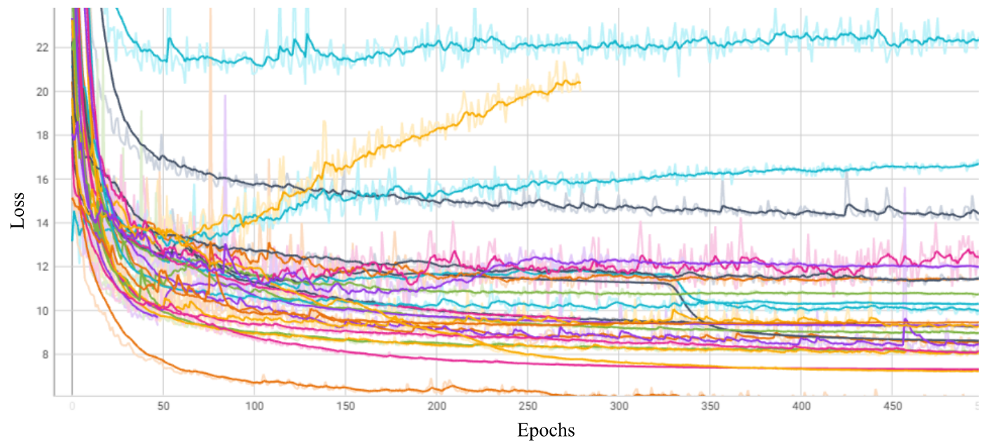
Several model architectures were tested in attempts to reach optimal performance. These architectures included XGBoost models, Deep Neural Networks (DNN) and Recurrent Neural Networks (RNN). These architectures were tested on a limited dataset and evaluated based on their ability to fit the provided data as well as their robustness on unseen data. From these tests it was determined that XGBoost models had the best ability to fit the response spectra but they were also less robust than DNNs. RNNs were considered as response spectra visually seem like continuous functions, however, in these tests RNNs yielded no increase in performance over DNNs. From a theoretical standpoint this aligns with the computational methods used in structural engineering, as each point on a response spectrum is calculated for an independent period and does not necessitate a smooth function. It was concluded that DNNs were the best choice for this study as they were not far behind the XGBoost models in ability to fit the data, and their increase in robustness made them the better choice. RNNs were not selected as they did not appear to provide significant benefit over DNNs and DNNs seemed like more fun at the time. Also the class this project started from was a Deep Learning class so... a DNN was chosen.

Once the model type was selected, hyperparameter tuning was carried out using the Keras Hyperband tuner to identify the optimal number of hidden units per layer as well as the level of regularization for each layer. This tuning was run for a number of different DNN model architectures with varying numbers of layers and regularization types (i.e. dropout, L1, and L2), yielding a total of eight distinct models. The training and validation losses were recorded in Tensorboard for ease of comparison and can be seen plotted in the figure below. Note that these losses have been smoothed for easier visualization, the unsmoothed values for each curve can be seen as a transparent layer behind each loss curve.

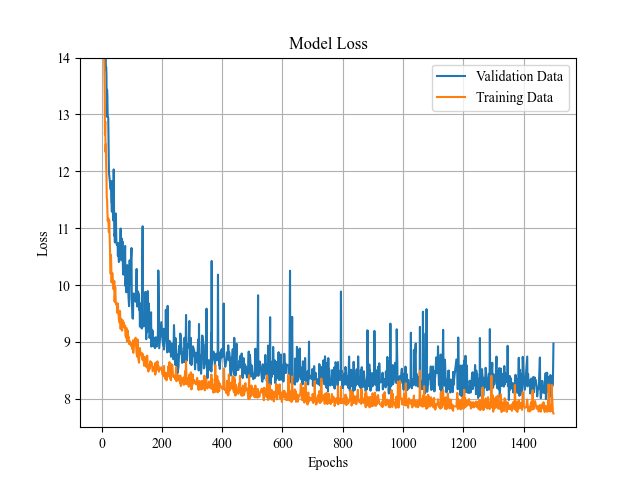
From these options, the optimal model was selected and training was continued for additional epochs to further decreasing the validation loss. The final model consisted of an eight layer DNN with L2 regularization. Both the number of hidden units and the regularization constant ramped up towards the middle layers and ramped back down towards the output layer. The unsmoothed loss curves for training and validation data can be seen in the figure below.

There are a couple things to note in this figure, the first being that there appears to be good convergence with a negative sloping trend, indicating that longer training may yield a more optimal model. However, I was training this model on my silly little desktop and 1500 epochs already took me awhile, so I called it a day (or several) after reaching this point. All models are checkpointed so in theory I could continue training where this left off, but I don't want to so... The next feature of note in this figure is the similarity in training and validation losses, while not perfect, this result was much better than many of the others models trained and it appeared to yield relatively robust predictions on the holdout dataset. To evaluate the model on the holdout test set, an evaluation metric of mean average percentage error was used for reasons previously stated. To assess the performance of the model, the Boore-Atkinson ground motion prediction equation was evaluated on the same holdout test set using the same metric for comparison. It is important to note that two tests were being run with the DNN, the first goal I had was to see if a DNN could recreate the Boore-Atkinson GMPE using the same inputs and no external knowledge of geomechanical phenomena, the second goal was to see if I could train a DNN that more accurately predicted response spectra, using additional input parameters. In the following table you can see the model performance of the Boore-Atkinson GMPE followed by the performance of the DNN using only the Boore-Atkinson input parameters (BSSA parameters), followed by the DNN using all available input parameters from the given database.

We can see that the DNN using only the BSSA input parameters achieves a very similar loss to that of the Boore-Atkinson GMPE, to me this indicates that the existing GMPE is highly tuned and provides an optimal solution for the given input parameters. This is not surprising as this was one of the most widely used ground motion prediction equations for many years and clearly had some smart people with big brains behind it. Nice job Boore and Atkinson! We can also see that when given additional inputs, the DNN is able to achieve a much lower loss than the previous models.

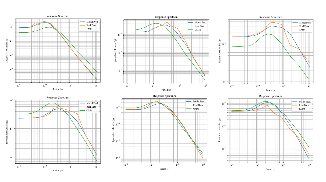
To visualize the outputs, I wanted to see how closely my DNN matched the actual response spectra and compare it to the BSSA GMPE. So I plotted a bunch of pictures and I will show you them now.

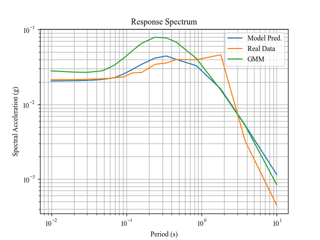
Here the green lines show the Boore-Atkinson GMPE and the blue lines depict the DNN performance (using all available parameters). The orange line shows the response spectra calculated using the accelerograms from the dataset and represent the ground-truth values for each seismic event. Although the DNN appears to more closely predict the response spectra, there are still several key ways the model is imperfect. The model is still unable to predict late period acceleration spikes, as can be seen in the figure below. Many existing GMPEs similarly struggle with this task and unfortunately, so does our new DNN friend.

This is problematic because it is underpredicting the effects of seismic events on structures with longer periods, which typically comprise of taller structures and long-span bridges, both of which can cause serious issues if damages. However, unusual spikes like these can often be attributed to more interesting soil conditions at the site of the accelerogram recording and are therefore more challenging to predict without additional data.

Future Work

Alright so if it was not clear by this point, I have written this in many different sittings, spanning many different moods, for the last bit I have been in a silly goofy mood, but I am not about to paste in a section that I wrote back in grad school when I was far less silly and far less goofy. I apologize for the solemnity of the following passage.

The purpose of a GMPE is to provide an attenuation relationship without requiring excessive amounts of effort. If the burden of collecting input feature data outweighs the benefit of using the GMPE, it no longer serves its purpose as an efficient calculation tool. For this reason, further investigation should be made into the features chosen for this analysis to conclude whether this is the case for the features in this model. Features such as hypocentral depth, PGA, and PGV (lol, if you are a Structural Engineer / Geotech you will realize how ridiculous it is to use PGA and PGV as inputs to a GMPE, but if you are neither of those, don't worry about it, those are super realistic and easy input variables and in no way bias the output of my DNN model...) may require intensive effort to calculate for unknown faults and therefore negate the usefulness of this model in realistic applications. Additionally, study into the covariance of the input parameters could help to eliminate unnecessary or redundant features. Lastly, alternate model architectures could be explored. The fact that the model performs better when predicting the entire response spectrum series (right sorry, this is something I have not yet mentioned and will not mention - get pranked, but basically, I tried to predict just a single point on the spectrum instead of predicting the entire spectrum all at once and it was like 10x slower and less accurate) seems to indicate dependence between points on the response spectrum. This information could be used to justify a recurrent neural network architecture, which may provide even better results (spoiler, it didn't - at least in my brief trials).

Conclusion

While the models presented in this study seem to indicate that using more parameters results in a more accurate model of ground motion attenuation, it is important to consider the tradeoff between collecting the data for these input variables and the desired level of model accuracy. As discussed in the Future Work section, some parameters used in the presented models may be very difficult to collect in practice, making the feasibility of using them potentially unrealistic. However, all models display similar or better performance than the baseline BSSA GMPE, indicating that machine learning frameworks can be used to predict ground motion attenuation without the model requiring any prior knowledge of geomechanical systems. This method shows promise as a feasible alternative to traditional GMPE development and will hopefully continue to be investigated by future researchers.

Ok thank you for reading :0)

References

[1] Boore, D. M., Stewart, J. P., Seyhan, E., and Atkinson, G. M. (2014). “NGA-West2 Equations for Predicting PGA, PGV, and 5% Damped PSA for Shallow Crustal Earthquakes.” Earthquake Spectra, 30(3), 1057-1085. http://www.earthquakespectra.org/doi/abs/10.1193/070113EQS184M

[2] Dhanya, J., and S. T. G. Raghukanth. "Ground motion prediction model using ar- tificial neural network." Pure and Applied Geophysics 175.3 (2018): 1035-1064. https://link.springer.com/article/10.1007/s11600-019-00395-yBib1

[3] Lake, T. (n.d.). 6 of the world's Deadliest Natural disasters. Encyclopædia Britannica. Re- trieved December 9, 2022, from https://www.britannica.com/list/6-of-the-worlds-deadliest- natural-disasters

[4] “Welcome to the Peer Ground Motion Database.” PEER Ground Motion Database - PEER Center, https://ngawest2.berkeley.edu/